
概述
本系列文章研究成熟的有限元理论基础及在商用有限元软件的实现方式。
有限元的理论发展了几十年已经相当成熟,商用有限元软件同样也是采用这些成熟的有限元理论,只是在实际应用过程中,商用CAE软件在传统的理论基础上会做相应的修正以解决工程中遇到的不同问题,且各家软件的修正方法都不一样,每个主流商用软件手册中都会注明各个单元的理论采用了哪种理论公式,但都只是提一下用什么方法修正,很多没有具体的实现公式。
商用软件对外就是一个黑盒子,除了开发人员,使用人员只能在黑盒子外猜测内部实现方式。
一方面我们查阅各个主流商用软件的理论手册并通过进行大量的资料查阅猜测内部修正方法,另一方面我们自己编程实现结构有限元求解器,通过自研求解器和商软的结果比较来验证我们的猜测,如同管中窥豹一般来研究的修正方法,从而猜测商用有限元软件的内部计算方法。
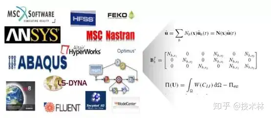
我们关注CAE中的结构有限元,所以主要选择了商用结构有限元软件中文档相对较完备的Abaqus来研究内部实现方式,同时对某些问题也会涉及其它的Nastran/Ansys等商软。为了理解方便有很多问题在数学上其实并不严谨,同时由于水平有限可能有许多的理论错误,欢迎交流讨论,也期待有更多的合作机会。
显式和隐式的区别
CAE求解方法一般有两种,分别为显式(Explicit)和隐式(Implicit)。显式求解算法基于动力学方程,当前时刻的位移只与前一时刻的速度和位移相关,求解过程中无需迭代;而隐式求解基于虚功原理,一般需要进行迭代计算。
在Abaqus中,显式求解和隐式求解一般都会采用增量求解,即将分析步分割为若干个增量步,在当前增量步达到平衡时计算下一个增量步。
1. 显式(Explicit)
在显式求解过程中,每个增量步内不需要进行迭代求解,且无需形成切线刚度矩阵,故每个增量步内计算量相对于隐式求解方法消耗较小,一般与单元规模成正比。但增量步长也不能过大,一般不超过模型最小自由振荡周期的1/10,否则容易导致计算结果发散。
2. 隐式(Implicit)
在隐式求解过程中,每个增量步都需要进行平衡迭代,需要形成切线刚度矩阵,计算量相对较大,一般与单元规模和迭代收敛速度相关。隐式求解的收敛速度和稳定性根据选择迭代方法的不同而不同。因此,需要针对模型特性选择合适的增量步长,保证计算结果的收敛。
综上,无论是显式求解还是隐式求解,都需要根据模型和求解问题合理设置分析步的增量步长和求解方法,保证分析的精度和质量。虽然这两种求解方法已经是有限元的基本动力学求解方法,但由于有限元本身的复杂性,往往很多人都难以理解两者的区别和显式为何发射,本文将以一个简单的算例配合代码实现来直观的解释一下隐式和显式的区别。
1.1 前向欧拉(Forward Euler)和后向欧拉(Backward Euler)
前向欧拉和后向欧拉分别是显式和隐式的一个典型计算方法,本文将引用这两个方法来尽量直观地展现显式求解和隐式求解的区别。
前向欧拉:
fn+1 (x) = fn (x) + h*f’n (x)
后向欧拉:
fn+1 (x) = fn (x) + h*f’n+1 (x)
1.2 算例
现在以一个微分方程算例为例:
y'(x) = -y+x+1
且有y(0) = 1。
1、前向欧拉法
使用前向欧拉法,可得:
yn+1 = yn + h*(-yn +xn +1)
显然,这个式子不需要做任何额外运算就能从yn出yn+1,因此每步迭代计算量小。但h在一个最大限制,具体见下面的推导过程:
yn+1 = (1-h)yn + h*(xn +1)
可得
yn+1 = (1-h)2 yn-1 + h*(xn +1) + h*(xn-1 +1)
则得
yn+1 = (1-h)n +O(s2 )
当h<2时,y收敛,但h>=2时,y将发散。
2、后向欧拉法
yn+1 = yn + h*(-yn+1 +xn+1 +1)
这个式子不能直接得出yn+1, 必须做进一步计算得到
yn+1 = (yn + h*(xn+1 +1)) / (1+h)
当h>0时,y无条件收敛。
3、结果比较
假设n=30
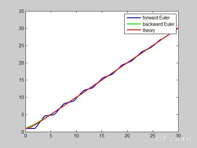
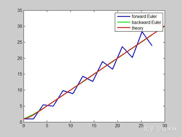
(1)当h = 1.9时,计算结果如下图所示,显式和隐式都和理论接近:
(2)当h = 2.1时,计算结果如下图所示,显式求解发散了:
总结
本文简单介绍了显式和隐式的区别,本质在于采用不同的物理学平衡方程,因此在不同的物理学问题也有不同的表现。文中给出一个数学算例,并分别利用前向欧拉和后向欧拉求解,以求直观表现显式和隐式在求解过程中的差异,以及增量步长对求解结果的影响。
What are the differences between implicit and explicit?
In static analysis, there is no effect of mass (inertia) or of damping. In dynamic analysis, nodal forces associated with mass/inertia and damping are included.
Static analysis is done using an implicit solver in LS-DYNA. Dynamic analysis can be done via the explicit solver or the implicit solver.
.
In nonlinear implicit analysis, solution of each step requires a series of trial solutions (iterations) to establish equilibrium within a certain tolerance. In explicit analysis, no iteration is required as the nodal accelerations are solved directly.
The time step in explicit analysis must be less than the Courant time step (time it takes a sound wave to travel across an element). Implicit transient analysis has no inherent limit on the size of the time step. As such, implicit time steps are generally several orders of magnitude larger than explicit time steps.
Implicit analysis requires a numerical solver to invert the stiffness matrix once or even several times over the course of a load/time step. This matrix inversion is an expensive operation, especially for large models. Explicit doesn’t require this step.
Explicit analysis handles nonlinearities with relative ease as compared to implicit analysis. This would include treatment of contact and material nonlinearities.
.
In explicit dynamic analysis, nodal accelerations are solved directly (not iteratively) as the inverse of the diagonal mass matrix times the net nodal force vector where net nodal force includes contributions from exterior sources (body forces, applied pressure, contact, etc.), element stress, damping, bulk viscosity, and hourglass control. Once accelerations are known at time n, velocities are calculated at time n+1/2, and displacements at time n+1. From displacements comes strain. From strain comes stress. And the cycle is repeated.